Seeing the Trees for the Forest | A gentle introduction to tree-based methods Part 1
Background & Motivation
As the title of this post suggests, I think there is great value in understanding, at a very low level, how decision trees are built. I hope to present a simple introduction of this process, and then build this out to trees and forests in future posts. But first, a little analogy that hopefully sets some intuition for how this works.
Do you remember playing the game “20 Questions” to pass the time during a long car ride or sleepless nights as a kid? For those that missed out, the game involved two people, a Questioner (Q) and and Answerer (A). First, A thinks of an object and keeps this selection private. Then, Q has the opportunity to ask 20 Yes/No questions in an effort to identify A’s secret object. If you are unfamiliar and curious, try it out here (excuse the clunky UI, and note that you will be playing against a computer Questioner).
When I first learned of the game, I remember being amazed/skeptical that someone could hone in on a specific object from the vast sea of possible words in a mere 20 questions. However, I soon learned that 20 questions was more than enough to identify most objects (at least, objects familiar to a 10 year old). Additionally, the particular questions I asked impacted how quickly and efficiently I could hone in on the target object (rather than just asking the same predefined 20 questions every game, for example).
Although at the time, I was not thinking of my gameplay as selecting “optimal questions” to efficiently “partition the object space”, in hindsight I realize I (needless to say, this is not specific to me, I would guess it applies to most kids who learn the game) internalized some of the same rules that, at an abstract level, govern how decision trees learn a problem.
The takeaway was: even simple yes/no questions, when chosen properly, can efficiently partition even a very complex space.
Decision Trees: Selecting Splits
Generating Candidate Splits
Similar to the questions in a game of 20 Questions, decision trees ask a series of Yes/No questions about your data. At each step, we first gather a list of all potential questions about our features (for categorical features, we can ask “Is Feature I = X” for each category X in Feature I, and for continuous features we can ask “Is Feature I greater than X” for each observed value of Feature I (or some discretization of the observed values)).
Suppose we have the following toy dataset of salaries by age and geographic region:
| Age | Region | Salary |
|---|---|---|
| 25 | West | 53 |
| 55 | West | 98 |
| 19 | Midwest | 50 |
| 49 | Midwest | 110 |
Given such a table, we can generate all candidate splits with the following code:
def get_candidate_splits(df, y):
    """
    df: pandas dataframe, to search for possible splits
    y: value we are trying to predict (so omit from candidate splits)
    """
    candidate_splits = []

    for col, dtype in df.dtypes.iteritems():
        if col == y:
            # We don't want to split on target variable
            continue
        if np.issubdtype(dtype, np.number):
            # If numeric, discretize cutpoints to be along the deciles (not a general rule, my simplification here)
            if df[col].nunique()<5:
                candidate_splits += [(col, v) for v in sorted(df[col].unique())[1:]]
            else:
                candidate_splits += [(col, v) for v in set(np.percentile(df[col].dropna(), range(10, 100, 10)))]
        else:
            # If categorical, split on the 10 most frequenty occuring values (again my simplification)
            if df[col].nunique()<10:
                candidate_splits += [(col, v) for v in df[col].unique()]
            else:
                candidate_splits += [(col, v) for v in df[col].value_counts().sort_values(ascending=False).index[:10]]

    return candidate_splits
Applying this to the toy dataset gives:
candidate_splits = get_candidate_splits(toy_data, 'Salary')
print(candidate_splits)
[('Age', 25),
('Age', 49),
('Age', 55),
('Region', 'Midwest'),
('Region', 'West')]
This tells us we can ask the following Yes/No questions of the dataset:
- Is the age < 25?
- Is the age < 49?
- Is the age < 55?
- Is the Region == Midwest?
- Is the Region == West?
Now that we have generated the set of candidate questions, we can turn to the issue of which question to ask in order to gain the most information about salary.
Selecting Optimal Split
Once we have generated all possible splits of our data, we need a decision rule to select the “best” split. This rule can take different forms, but in general we are trying to minimize some cost function of our data. In the classification context, the cost function often takes the form of average entropy within leaves across the tree. For regression, which we are exploring here, we can try to minimize variance of the target variable within groups. The goal is to split the data in such a way that the resulting groups are as “similar” as possible (with regards to some specified target variable).
Suppose we start with some group X and variable y. Then, we can generate various splits of X according to each of the candidate splits identified in the previous section, to get resulting groups X_i and X_j. For each of these splits, we can calculate a new weighted variance as follows:
def get_split_variance(X, feature, val, y):
    if np.issubdtype(X[feature].dtype, np.number):
        X_i = X.loc[X[feature] < val]
        X_j = X.loc[X[feature] >= val]
    else:
        X_i = X.loc[X[feature] == val]
        X_j = X.loc[X[feature] != val]

    return ((np.var(X_i[y]) * X_i.shape[0]) + (np.var(X_j[y]) * X_j.shape[0])) / X.shape[0]
This is simply a function of the dataframe (X), split information (feature and value), and target variable (y). Thus, we can easily calculate the resulting weighted variance of every candidate split, and then select the split that results in the lowest weighted variance (equivalently, the split with greatest variance reduction from the original X).
Applying this to our toy dataset and candidate splits, we get the following variance reduction for each split:
def get_variance_reduction(df, candidate_splits, y):
    variance_reductions = []
    for split in candidate_splits:
        variance_reductions.append((split[0], split[1], get_split_variance(df, split[0], split[1], y)))

    var_df = pd.DataFrame(variance_reductions, columns=['feature', 'value', 'variance'])
    var_df['variance_reduction'] = df[y].var() - var_df['variance']

    return var_df.sort_values('variance_reduction', ascending=False)

get_variance_reduction(toy_data, candidate_splits, 'Salary')
This results in the following split stats:
| feature | value | variance | variance_reduction |
|---|---|---|---|
| Age | 49 | 19.125 | 925.125 |
| Age | 25 | 451.5 | 492.75 |
| Age | 55 | 571.5 | 372.75 |
| Region | Midwest | 703.125 | 241.125 |
| Region | West | 703.125 | 241.125 |
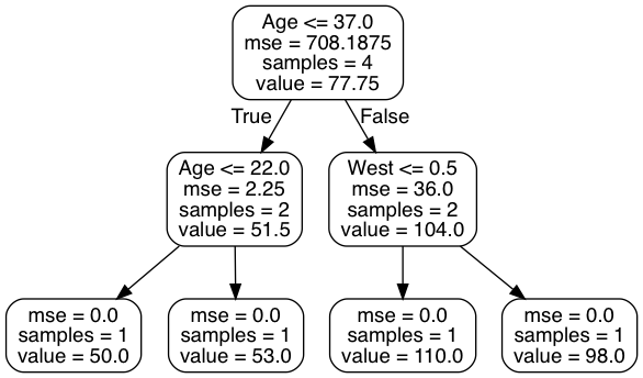
This tells us that our first split should be on Age >= 49, as that will lead to the largest reduction of variance for the
Salary variable. You can probably see that this will result in two new datasets X_i and X_j, each of which have
their own set of candidate splits and associated variance reductions. In this way, we can recursively apply the
algorithm on the subgroups until some stopping criterion is met (e.g. commonly a maximum “depth” or some minimum required
number of samples). The resulting model has a tree structure, where predicting the target for a new sample involves
traversing the Yes/No questions until reaching a final terminal node, at which point the prediction is the average (or
modal, in the case of classification) value target value of training data that ended up in that node.
The following image provides a visualization of the resulting model structure (note that the particular split points are slightly different, based on how scikit chooses splits vs. how I did, but result in the same groups for our training data, e.g. Age <= 37.5 results in the same split as Age < 49 /Age >= 49 in our data).
As a final, I will demonstrate the flexibility of the approach on a more real dataset, so the results are perhaps more interesting and compelling.
male_wages = pd.read_csv('https://vincentarelbundock.github.io/Rdatasets/csv/plm/Males.csv').drop(['Unnamed: 0', 'nr'], axis=1)
male_wages.head()
| year | school | exper | union | ethn | married | health | wage | industry | occupation | residence |
|---|---|---|---|---|---|---|---|---|---|---|
| 1980 | 14 | 1 | no | other | no | no | 1.19754 | Business_and_Repair_Service | Service_Workers | north_east |
| 1981 | 14 | 2 | yes | other | no | no | 1.85306 | Personal_Service | Service_Workers | north_east |
| 1982 | 14 | 3 | no | other | no | no | 1.34446 | Business_and_Repair_Service | Service_Workers | north_east |
| 1983 | 14 | 4 | no | other | no | no | 1.43321 | Business_and_Repair_Service | Service_Workers | north_east |
| 1984 | 14 | 5 | no | other | no | no | 1.56813 | Personal_Service | Craftsmen, Foremen_and_kindred | north_east |
Looking at a sample of candidate splits:
pd.DataFrame(get_candidate_splits(male_wages, 'wage')).drop_duplicates(0).values

 ['year' 1983.5]
 ['school' 10.0]
 ['exper' 8.0]
 ['union' 'no']
 ['ethn' 'other']
 ['married' 'no']
 ['health' 'no']
 ['industry' 'Manufacturing']
 ['occupation' 'Craftsmen, Foremen_and_kindred']
 ['residence' 'south']
Sorting splits by resulting variance reduction:
| feature | value | variance | variance_reduction |
|---|---|---|---|
| school | 12.0 | 0.267075 | 0.0165982 |
| year | 1983.5 | 0.268026 | 0.0156472 |
| year | 1985.0 | 0.269613 | 0.0140595 |
| year | 1982.0 | 0.270806 | 0.0128672 |
| school | 11.0 | 0.271068 | 0.012605 |
| married | no | 0.271655 | 0.0120179 |
| married | yes | 0.271655 | 0.0120179 |
| exper | 5.0 | 0.27271 | 0.0109627 |
| exper | 6.0 | 0.273995 | 0.00967737 |
| school | 14.0 | 0.274754 | 0.00891904 |
Thus we would expect the first split to be on whether schooling is greater than or equal to 12. Sure enough, we can fit this data with scikit and inspect the resulting tree, where the first split splits the group into those with 12 or more and less than 12 years of schooling, respectively.
from sklearn.ensemble import DecisionTreeRegressor

X = male_wages_w_dummies.drop(cat_cols+['wage'], axis=1)
dtr = DecisionTreeRegressor().fit(X, male_wages_w_dummies['wage'])

export_graphviz(dtr, out_file=out_f,
               feature_names=X.columns.tolist(),
                max_depth=3,
                rounded=True,)

Next Steps
In a future post, I will go more into the details such as how we decide on a stopping criterion, limitations to the decision tree framework, and how extensions like bagging and random forests can address some of these shortcomings. In this post, I wanted to lay the groundwork for thinking about how a tree is constructed at the most micro level. Breaking it down into components like “candidate split search” and “optimal split selection” also lay a good foundation for reasoning about model training and parameter tuning. For example, as we will see when we move into random forests, limiting the candidate split search to a random subset of the features at each split can significantly improve model test performance and generalizability. Or we may want to modify the selection step; for certain applications our notion of “best split” may involve another metric such as MAE that is less sensitive to outliers.