Hypothesis Testing: From T to Z
Background & Motivations
With all the modern tools for stats, it is easy to treat many of the methods as black boxes. As such, I had often felt unsatisfied with my understanding of the nuances of hypothesis testing. I took enough psychology and research design courses to understand the general motivation: given two groups and some observed variable, one can apply statistical tests to determine whether the groups are “meaningfully different” to some specified confidence level. However, my limited exposure to the statistical basis meant I treated the method as a black box that magically returned a number (hopefully less than .05 😅), with little underlying sense of exactly when, how, or why it worked.
About a year ago, I came across a PyCon video I would highly recommend called Statistics for Hackers. His underlying message: "If you can write a for-loop, you can do statistics" I had never seen the materials presented in this way; seeing the concepts presented in concrete code made the ideas click in a way that reading stat formulas never had (very similar to the effect of the Hacker’s Guide to Neural Networks, a topic for another post).
More recently, a coworker presented a Lunch & Learn that went a bit further, connecting dots between the “hacker’s” perspective and a more traditional statistician’s approach. Then, I took the time to actually code out some of the details, and the concepts started to become much more clear. I won’t go into the nitty gritty details of hypothesis testing here, as there are many readily available resources on the web. However, I will provide a high level overview that will hopefully orient the reader and provide some context to this code. In the remainder of this post, I will present my short “hacker’s guide” to t-testing.
Setting Up the Problem
Suppose you have two groups (let’s say “data scientists” and “data analysts” in Philadelphia), and you want to know whether some observed variable X (e.g. average salary) is different between these two groups.
Let us first assume that I am collecting the data by hand and I am feeling lazy, so only randomly collect 8 data points from each group (using statistically sound sampling methods, of course). Here is the data:
| Data Scientists | Data Analysts |
|---|---|
| $92,560.75 | $68,424.92 |
| $48,881.98 | $95,407.34 |
| $110,757.97 | $76,322.59 |
| $91,586.44 | $78,782.42 |
| $80,829.60 | $112,623.09 |
| $118,819.84 | $82,237.21 |
| $103,788.47 | $34,663.55 |
| $105,281.72 | $67,206.20 |
We want to know if there is a significant difference between salaries of the two groups.
If we look at the group means, we see that data scientists in this sample made an average of $94k, while data analysts made ~$77k on average. While this intuitively seems like a large difference, there is a chance we got “unlucky” and happened to sample data scientists at the higher end of the pay-scale (or analysts at the lower end, or both). Hypothesis testing allows us to more rigorously answer this question, by quantifying how likely we are to observe the difference by chance, assuming no true difference between the groups.
Test Statistics
A test statistic is simply a quantity derived from a sample. We can calculate different test statistics from these samples above.
Both of these statistics will involve comparing the difference in group means relative to the variance of the sampling mean (not to be confused with the variance of the underlyinh population itself). The variance is a measure of the spread of datapoints from a mean. So as this becomes larger, so too does the likelihood of observing larger differences between sample means.
If we know the true underlying population variance (uncommon situation, but with large N, the sample approximation is often good enough) we can calculate a z-statistic, which measures the amount of between group variance relative to the within group variance.
The t-statistic provides another measure of between / within group variance, but can be used when the population variance is unknown, and corrects for the fact that the sample variance is an estimate of the population variance with it’s own associated standard error. This distinction becomes less important as the sample size increase, and thus the sample variance approaches the population variance, but can have an impact in scenarios with small sample size, as we will see below.
Writing Some Code
First, we will code up the calculation of the aforementioned statistics. You can see the details for yourself here and elsewhere.
We will define some common shared methods: standard error is a measure of the standard deviation of the sampling mean, calculated as:
def standard_error(std, n):
    # std: standard deviation of the population
    # n: number of observations in sample
    return std / np.sqrt(n)
Because we are comparing two groups in an independent samples t-test, we need to calculate the standard error of the new distribution G1 - G2. We can do that as:
def standard_error_of_difference(g1, g2, std):
    standard_errors = list(map(lambda grp: standard_error(std, len(grp)), [g1, g2]))
    return np.sqrt(np.sum(np.square(standard_errors)))
Our z-score, then, can be calculated as:
def zscore(g1, g2, std):
    standard_error = standard_error_of_difference(g1, g2, std)
    return (g1.mean() - g2.mean())/standard_error
If we do not know the true population standard deviation, we estimate it from pooling sample as follows:
def pooled_sigma(g1, g2):
    pooled_var = sum([(len(grp) - 1)*grp.var(ddof=1) for grp in [g1, g2]]) / (len(g1) + len(g2) - 2)
    return np.sqrt(pooled_var)
For a t-test (where we don’t know the population standard deviation), we can calculate the t-score as:
def tscore(g1, g2):
    estimated_std = pooled_sigma(g1, g2)

    standard_error = standard_error_of_difference(g1, g2, estimated_std)
    return (g1.mean() - g2.mean())/standard_error
The two calculations are very similar. We can explicitly see how they are related with the following function:
def test_statistic(g1, g2, std=None):
    # if std provided, calculates z-score.
    # else, estimates population SD and calculates t-score
    if std is None:
        # Population variance not known. Calculate t-stastic
        std = pooled_sigma(g1, g2)

    se = standard_error_of_difference(g1, g2, std)

    return (g1.mean() - g2.mean()) / se
Calculating the Test Statistics
If we perform a z-test (thus assuming we know the population standard deviation), we get a z-score of -1.520, which corresponds to a p-value of .129 (cdf of the standard normal, x2 for both tails). This means that if there were no difference between salaries of the two groups, I would see a between-group difference of equal or greater magnitude than the currently observed difference a little under 13% of the time, just from variance in the sample mean.
z = test_statistic(g1, g2, np.concatenate([g1, g2]).std())
print(z, norm.cdf(z)*2)
=> prints `-1.519694634779407 0.12858774066981019`
However, suppose more realistically that I do not know the underlying variance of salaries in the population. In this case, my p-value should account for the uncertainty introduced by the population variance estimate. When I perform a t-test, I get a t-statistic of -1.537, which corresponds to p=0.147 for this sample size, meaning I would actually expect to see this magnitude of difference (or greater) under the null hypothesis just under 15% of the time.
t = test_statistic(g1, g2)
p = stats.t.cdf(t,df=size*2-2)*2
print(t, p)
=> prints `-1.5367748542943334 0.14663716542911295`
What we’ve seen is the following: if I did not know the true underlying standard deviation (as I likely wouldn’t in practice), incorrectly applying the z-test would lead to an over-confidence that the observed difference is significant. In both cases here, we cannot reject the null hypothesis with much confidence. But, if for some strange reason we had set out confidence level to 13%, the z-test would result an unjustified rejection of the null hypothesis.
Validating & Visualizing Results
First, let’s consider how we could empirically assess the significance levels that were calculated analytically up above. The critical idea here is that the test-statistic will take a particular distribution when there is no true difference between the two groups, and we can model this distribution by repeatedly repeatedly pooling the two groups and resampling and re-calculating the test statistics. We can do this as follows:
pooled = np.concatenate([g1, g2])
t = test_statistic(g1, g2)
z = test_statistic(g1, g2, pooled.std())

total = 0
larger_z = 0
larger_t = 0

zs = []
ts = []

for s in range(20000):
    sample_g1 = np.random.choice(pooled, replace=True, size=size)
    sample_g2 = np.random.choice(pooled, replace=True, size=size)

    sample_z = test_statistic(sample_g1, sample_g2, pooled.std())
    sample_t = test_statistic(sample_g1, sample_g2)

    zs.append(sample_z)
    ts.append(sample_t)

    if abs(sample_z) > abs(z):
        larger_z += 1
    if abs(sample_t) > abs(t):
        larger_t += 1
    total += 1

percent_larger_z = 100*float(larger_z)/total
percent_larger_t = 100*float(larger_t)/total

print(('Resampling 20k times under null hypothesis.'\
	'Proportion of test statistics greater than observed magnitude:\n'\
	'T: {:.2f}%\nZ:{:.2f}%'.format(percent_larger_t, percent_larger_z)))
Resampling 20k times under null hypothesis.
Proportion of test statistics greater than observed magnitude:
T-Stat: 14.56%
Z-Stat: 12.70%As we can see from the simulation above, resampling the data under the null hypothesis results in 14.56% of simulations with a t-stat greater than the observed value, and 12.70% where the z-value is greater. This is quite close to the analytic values we calculated above.
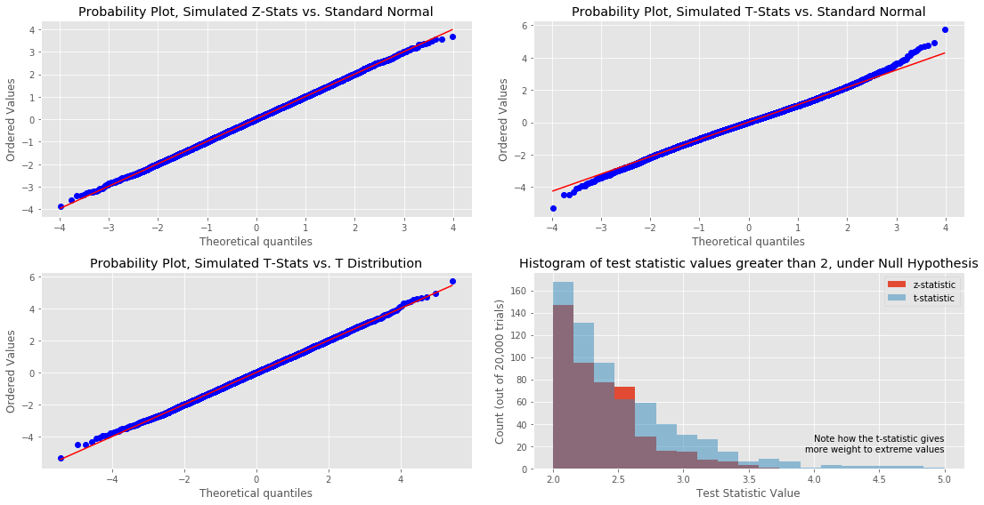
Finally, for a little insight into what is happening here, we can visually inspect how closely the simulated distributions match various theoretical distributions. As we can see below, the z-stat follows the standard normal distribution quite closely, whereas the t-stat diverges from the standard normal at the tails. However, when we plot against the relevant t-distribution, which accounts for the error introduced by estimating the population standard deviation with the sample, we see a much closer match at the tails of the distribution. Furthermore, in the lower right graph, we see that t-distribution results in a greater mass at the tail of the distibution.
Conclusions
This is probably not particularly revelatory for anyone with much of a statistics background, but I found the excercise of putting the concepts into code to be very helpful to my understanding. In particular, simulating the test statistics under the null hypothesis and working with a concrete sample of that statistic made concepts like the p-value (just the portion of the simulated values greater than the observed value) and why t- vs. z- for small samples (in the plots at the end, we clearly can see that the t-stat results in more mass at the tails of the distribution, which are underestimated with the z).
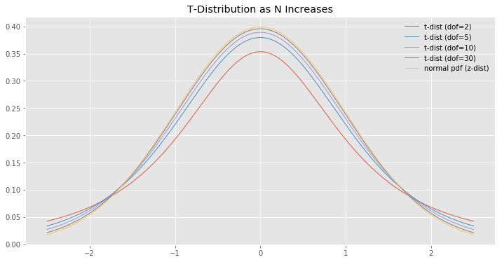
There is more I could write and present (e.g. show how t-dist converges to z-dist as the sample size increases), but there is always more, and I wanted to force myself to get something out there and start the ball rolling on this blog.